HSQC – Revealing the direct-bonded proton-carbon instrument

2D NMR experiments provide chemists with evidence to clarify and confirm resonance assignment. Nowadays every organic chemist uses these experiments called COSY, HMBC and HSQC as routine analytics. Basically, with 2D experiments you correlate some kind of information between two 1D spectra. If we correlate two 1D spectra of the same nucleus we are dealing with homonuclear 2D NMR experiments. The most famous representative of this group is the COSY experiment (find theory here and application here). Whereas, if we correlate 1D spectra of different nuclei, we call this heteronuclear 2D NMR correlation. One of the first heteronuclear 2D experiments invented was the HETCOR, a carbon detected experiment that was largely replaced by the HSQC (Heteronuclear Single Quantum Correlation) experiment. This provides the same information, but it is proton detected so you get that information faster! If you perform an ¹H,¹³C-HSQC you will find the ¹J_CH couplings, which means that the HSQC reveals which proton is directly bond to which carbon. Pretty useful, right?

Like every other 2D NMR pulse sequence the one used for HSQC consists of three parts (figure 1). Preparation, evolution (t1) and mixing. Subsequent to those we have the acquisition time (t2) in which the FID is detected. If you’ve dealt with other pulse sequences before, you might recognise the INEPT sequence (90-180-90 on one, 180-90 on the other channel) in the beginning of this pulse program. This is the preparation phase. The evolution takes place on the ¹³C spins while an 180° pulse is only applied on the ¹H channel. In the mixing period, there is another spin echo sequence which transfers the evolved information back to ¹H and is detected on this channel. For historic reasons, this is called an ‘inverse’ correlation. The advantage is, that we detect the signal on the more sensitive proton channel. If you want to know more about the pulse program, I can highly recommend Dr. James Keeler’s ‘Understanding NMR Spectroscopy’^[1] to you. This is the source, I gained most of my knowledge about pulse programs.

Figure 1. HSQC pulse sequence.[2]

For 1D experiments, the spectra have the chemical shift on the abscissa and the intensity on the ordinate. In 2D spectra you will find 3 axes. On two of them, called the F2 and F1 axis, the 1D spectra of each nucleus is plotted. The third axis is the intensity that directs out of the window plane. Important to understand is that in every 2D experiment the evolution time t1 is varied from t1 = 0 to nΔ (where n is integer). That means that you record an array of spectra. By that, one might understand that you cannot just run a regular Fourier Transformation (FT) just like for 1D spectra, but actually, its not so very different. Without going too much into details here, you have to do the FT twice. One along the F2 axis and another along the F1 axis. Once done you will receive a contour plot, which looks like reading an elevation map or isobars in the weather map – haha.

In figure 2 the HSQC spectrum of the indometacin (1) is depicted, recorded on our NMReady-60PRO in under 2 hours.

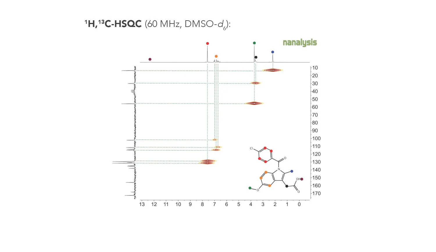
Figure 2. HSQC NMR spectrum of indomethacin (1).

Again, with HSQC you will find signals in the contour plot with the chemical shift of proton and carbon, which are directly bond. With HSQC we can assign all proton and all carbon signals except quaternary ones (naturally, as there is no ¹J_CH coupling, as there is no proton attached). Let’s go through it from downfield to upfield in the proton spectra (I added some comments in italic):

12.36 (s, 1H, CO₂H, not attached to any C, so no HSQC signal),
7.64 (bs, 4H, ClCq(CH_ArCH_Ar)₂, coupling to two high intensity carbon signals in the aromatic region, representing 4 carbon atoms, each 2 symmetrical),
7.08-6.59 (m, 3H, MeOCq(CH_Ar)₂, NCqCHAr, as this benzene ring is not symmetrically substituted, one finds different shifts for each CH_Ar carbon),
3.77 (s, 3H, OCH₃, in comparison with the other CH₃ group in the molecule, this methoxy group clearly is shifted downfield, so the assignment is with no doubt),
3.67 (s, 2H, HO₂CCH₂),
2.24 (s, 3H, NCqCH₃).

Cool, huh? One experiment and the protons are fully characterized, and the carbons are almost done, as well. For the assignment of the quaternary carbons on might consult a ¹H,¹³C-HMBC spectrum...let’s keep that one for another session.

References
^[1]http://www-keeler.ch.cam.ac.uk/lectures (accessed February 2019).
^[2]Riegel, S. D.; Leskowitz, G. M. TrAC, 2016 8327-38