Your Nanalysis 60 Order!

The spectra were analyzed according to first order’. Does this sound familiar to you? Most of the supporting information documents out there contain this sentence. You find yourself asking ‘why does nobody care about second order effects?’, then check out this high-order blog entry on the topic.

First, let’s point out what we are dealing with here. First order can be roughly described as the ability to look at a spectrum and visually extract the information. Second, and higher order effects mean that while the information is still contained in the spectra, it may be too convoluted for you extract manually.

Second order effects in NMR spectroscopy occur when the difference in chemical shifts (Δv [in Hz] not Δδ [in ppm] so we can compare directly) of two resonance, which have similar values to the corresponding scalar coupling (J [Hz]) of those signals. This can be expressed by equation (1), which can be easily transformed to equation (2).^[1]

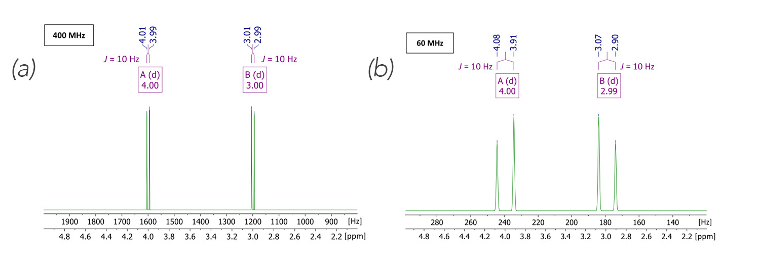
Figure 1. Simulated first order (Δv > 5J) spectra[2] in a high (left) and low (right) magnetic field, respectively. Parameters of choice: AB spin system; δ[ppm] = 4.00, 3.00; J1 = 10 Hz; spectral width = 2 to 5 ppm; spectrometer frequency = 400 MHz (left), 60 MHz (right); number of points = 16k. For clarity, two f1-axes, one with the dimension of Hertz, the other in ppm are displayed

To visualize this theoretical approach, I’d like to utilize an NMR simulation tool provided by nmrdb.org.^[2] In Figure 1, two spectra are illustrated describing a (mostly) first order situation. In both the 400 and 60 MHz spectra shown, the chemical shift was chosen to be δ[ppm] = 4.00 and 3.00.

In both of these cases the Δδ = 1 ppm, but when we convert that to the chemical shift in frequency on the 400 MHz spectrometer the difference in chemical shift is Δv = 400 Hz whereas at 60 MHz, the difference in chemical shift is only Δv = 60 Hz. With a chosen scalar coupling of J = 10 Hz for the high field case we can calculate a ratio Δv/J = 40, whereas in the case of the low field we get a ratio of Δv/J = 6.

We now want to set an unambiguous second order scenario. The distances of the chemical shifts of the two signals in the simulated spectra, displayed in figure 2 are much smaller now. The shifts were set to δ[ppm] = 3.55, 3.45 (i.e., Δδ = 0.1 ppm), the scalar coupling was maintained at J = 10 Hz, then we get a ratio of Δv/J = 4 and Δv/J = 0.6, respectively. This time the requirement of equation (2) is true for both examples and we would expect second order effects here. In fact, we do observe a strong roofing effect in the high field spectrum; wheras in the low field spectrum we find that the resonances overlap, resulting in a second order effect signal shape.

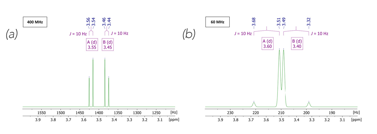
Figure 2. Simulated second order (Δv < 5J) spectra[2] in a high (left) and low (right) magnetic field, respectively. Parameters of choice: AB spin system; δ[ppm] = 3.55, 3.45; J1 = 10 Hz; spectral width = 3 to 4 ppm; spectrometer frequency = 400 MHz (left), 60 MHz (right); number of points = 16k. For clarity, two f1-axes, one with the dimension of Hertz, the other in ppm are displayed.

So far, we can conclude, that second order effects are more likely to be observed in NMR spectra acquired from a low field instrument, as Δv is by nature smaller compared to a high field instrument. But what about the nature of the actual compound we are observing? Let us transfer this to a real-life NMR experiment. Typically, substances with nuclei that are chemically equivalent but magnetically non-equivalent cause spectra with second order effects.^[3] Taking this into account, 3,4-dimethoxybenzaldehyde (1) could be a good candidate. For this reason, I acquired low and high field data for this compound. Let us take a look at the low field spectra first, recorded on the Nanalysis 60 (figure 3).

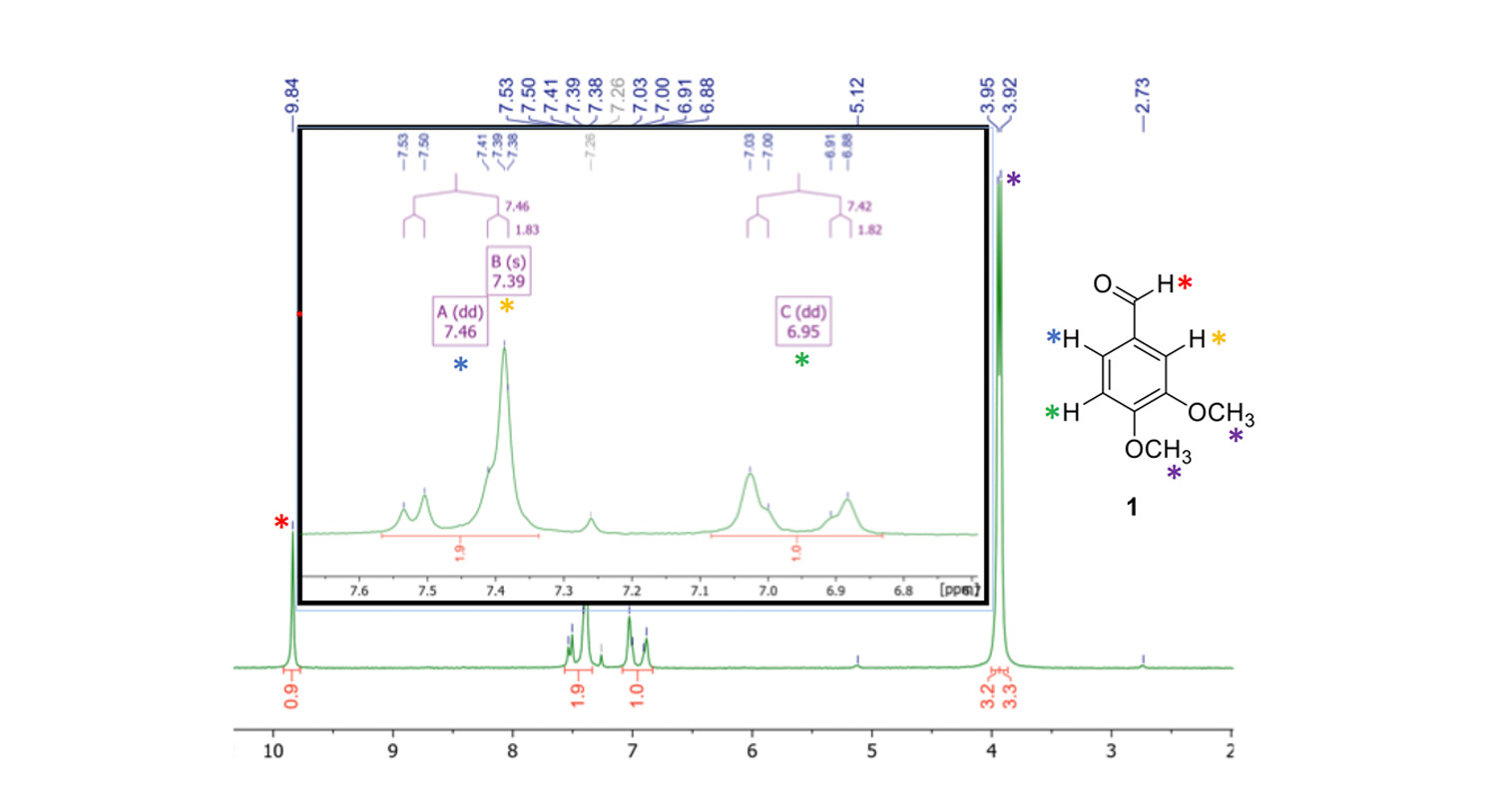
Figure 3. 1H NMR spectrum of 3,4-dimethoxybenzaldehyde (1) in CDCl3, recorded on a NMReady-60 at 60 MHz. Second order effects were clearly observed.

The aldehyde 1 can be unambiguously characterized with the low field NMR data. The aldehyde H-atom, as well as the aliphatic methoxy-group signals can be assigned easily (red and purple asterisks, figure 3). In fact, we do observe second order effects in the aromatic region, with a roofing effect where the peaks tend to point to each other and the intensity is not quite what you’d expect. Although we have an overlap of signal ‘B’ (yellow asterisk, δ = 7.39 (s, 1H, C(CHO)CHC(OCH₃)) ppm) and signal ‘A’ (blue asterisk, δ = 7.46 (dd, ^3/4J_HH = 7.5, 1.8 Hz, 1H, C(CHO)CHCH) ppm), I was still able to collect the scalar coupling constants here. For signal C (green asterisk, δ = 6.95 (dd, ^3/4J_HH = 7.4, 1.8 Hz, 1H, C(CHO)CHCH) ppm), we also observe a ‘second order-ish’ signal shape, but again, integral and J couplings have the right values.

So, although we’ve encountered second order effects with this substrate, we were able to get every information needed from the low field spectrum. For comparison I acquired high field data of the exact same sample on a 400 MHz instrument (figure 4).

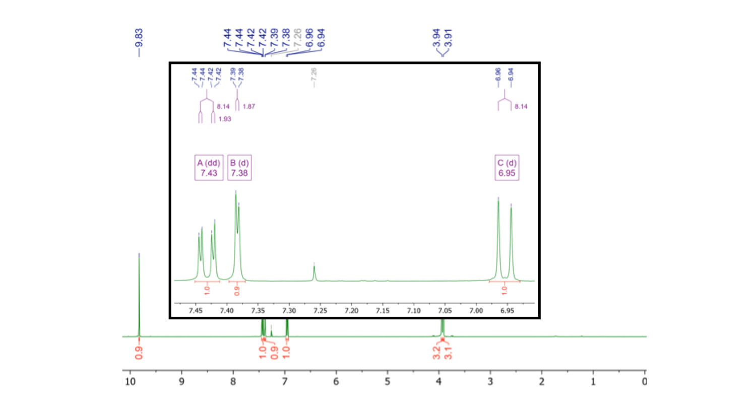
Figure 4. 1H NMR spectrum of 3,4-dimethoxybenzaldehyde (1) in CDCl3, recorded on a 400 MHz high field instrument. There are some slight roof effects, but not too much second order effects are going on here.

In the high field spectrum, the signals 'A' and 'B' are not overlapping and signal 'B' reveals to be a doublet instead of a single – the ⁴J coupling was not observed in the low field spectrum. The signal 'C' appears as a doublet instead of a doublet of doublets with the ⁴J coupling constant, as observed at 60 MHz.

In summary, although low field NMR spectra tend to show second order effects, one still can characterize the substance of interest. Of course, at some point, multiplet analysis will be even more challenging and one would have to get back to high field information OR you could try to find the coupling constants by JRes NMR Spectroscopy for those cases.

This is an important topic when it comes to benchtop NMR and low-field NMR spectroscopy, so we will continue to discuss this in future blog entries where we highlight how you can either embrace or ignore second order effects when using these 60 MHz instruments!

^[1]H. J. Reich, Chem 605 - Structure Determination Using Spectroscopic Methods, 2018, University of Wisconsin: https://www.chem.wisc.edu/areas/reich/nmr/05-hmr-09-2ndorder.htm (accessed October 2018)
^[2]a)A. M. Castillo, L. Patiny, J. Wist, J. Mag. Reson. 2011, 209, 123-130;
^b)https://www.nmrdb.org/simulator/index.shtml?v=v2.87.7 (accessed October 2018); Spectra were downloaded as jcamp txt files from the cited website and processed with Mnova.
^[3]https://www.ucl.ac.uk/nmr/NMR_lecture_notes/L3_3_97_web.pdf (accessed October 2018).